1
2
3
4
5
6
7
8
9
10
11
12
13
14
15
16
17
18
19
20
21
22
23
24
25
26
27
28
29
30
31
32
33
34
35
36
37
38
39
40
41
42
43
44
45
46
47
48
49
50
51
52
53
54
55
56
57
58
59
60
61
62
63
64
65
66
67
68
69
70
71
72
73
74
75
76
77
78
79
80
81
82
83
84
85
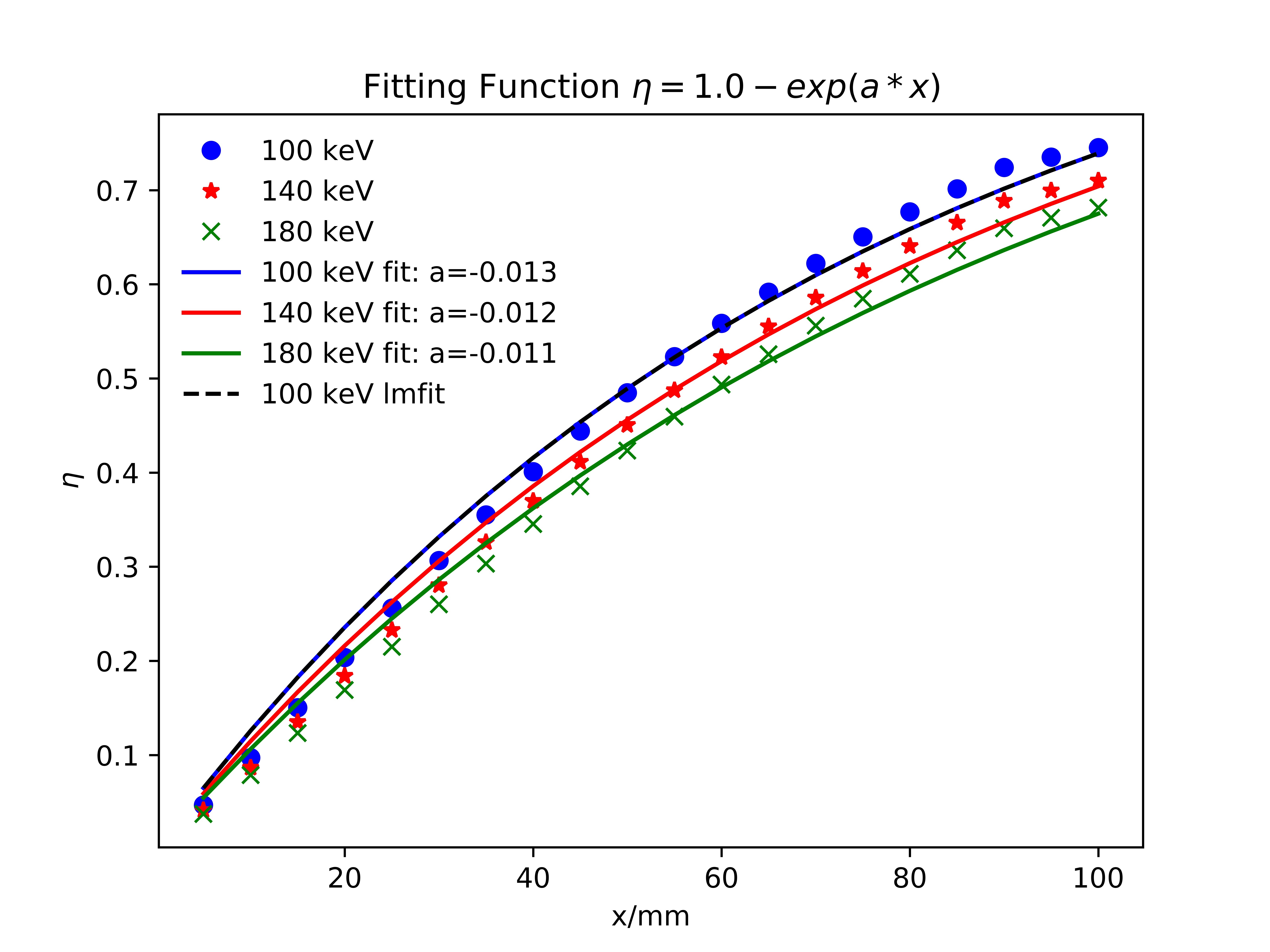
|
import numpy as np
import matplotlib.pyplot as plt
from scipy.optimize import curve_fit
from lmfit import Model
def func(x, a):
return 1. - np.exp(a * x)
x = np.linspace(5, 100, 20)
y1 = np.loadtxt('dataout1.txt')
y2 = np.loadtxt('dataout2.txt')
y3 = np.loadtxt('dataout3.txt')
plt.plot(x, y1, 'bo', label='100 keV')
plt.plot(x, y2, 'r*', label='140 keV')
plt.plot(x, y3, 'gx', label='180 keV')
popt1, pcov1 = curve_fit(func, x, y1)
plt.plot(x, func(x, *popt1), 'b-',
label='100 keV fit: a=%5.3f' % tuple(popt1))
popt2, pcov2 = curve_fit(func, x, y2)
plt.plot(x, func(x, *popt2), 'r-',
label='140 keV fit: a=%5.3f' % tuple(popt2))
popt3, pcov3 = curve_fit(func, x, y3)
plt.plot(x, func(x, *popt3), 'g-',
label='180 keV fit: a=%5.3f' % tuple(popt3))
gmodel = Model(func)
result = gmodel.fit(y1, x=x, a=-0.02)
print(result.fit_report())
plt.plot(x, result.best_fit, 'k--', label='100 keV lmfit')
plt.title(r'Fitting Function $\eta = 1.0-exp(a*x)$')
plt.xlabel('x/mm')
plt.ylabel(r'$\eta$')
plt.legend()
leg = plt.legend()
leg.get_frame().set_linewidth(0.0)
plt.savefig('myfit.jpg', format='jpg', dpi=1000, figsize=(8, 6), facecolor='w', edgecolor='k')
|